Why You Should Use Apache Iceberg with PySpark ?

If you’ve had experience with data lakes, you likely faced significant challenges related to executing updates and deletes. Managing the concurrency between multiple readers and writers, addressing schema evolution in your data, and managing the partitions evolution when data volumes or query patterns change.

In this article, we will explore how to use Apache Iceberg with PySpark to address these challenges.

What is Apache Iceberg?

Apache Iceberg is an open table format designed for extensive analytics datasets. It is compatible with widely used big data processing engines such as Apache Spark, Trino, PrestoDB, Flink, and Hive.

Iceberg tackles several limitations we listed above by acting as a metadata layer on top of the file format like Apache Parquet and Apache ORC. The following key features of Iceberg effectively address these limitations:

Schema Evolution: Allows for seamless schema evolution, overcoming the challenges associated with changes in data structure over time.
Transactional Writes: By supporting transactional writes, Iceberg ensures the atomicity, consistency, isolation, and durability (ACID) properties, enhancing data integrity during write operations.
Query Isolation: Iceberg provides query isolation, preventing interference between concurrent read and write operations, thus improving overall system reliability and performance.
Time Travel: The time travel feature in Iceberg allows users to access historical versions of the data, offering a valuable mechanism for auditing, analysis, and debugging.
Partition Pruning: Iceberg’s partition pruning capability optimizes query performance by selectively scanning only relevant partitions, reducing the amount of data processed and improving query speed.

Now, let’s start exploring how Iceberg facilitates the implementation of these features when combined with PySpark.

Install required dependencies

python -m venv iceberg
source gx/bin/activate
pip install pyspark==3.4.1

Before you start working with Apache Iceberg and PySpark, you need to install the necessary dependencies. Run the commands below to create a virtual environment called iceberg (or choose any name you prefer), activate it, and then install pyspark dependency.

Note: If you are using Windows, run the command .\iceberg\Scripts\activate to activate the virtual environment.

The versions employed in this article are:

Python: 3.11.6
PySpark: 3.4.1

Import required packages

Once you install the dependencies, import the necessary packages that you will use in the following sections.

from pyspark.sql import SparkSession
from pyspark import SparkConf
from pyspark.sql.types import StructType, StructField, StringType, IntegerType

Setup Iceberg Configuration

To begin working with Iceberg tables in PySpark, it’s essential to configure the PySpark session appropriately. In the following steps, we will use a catalog named demo for tables located under the path ./warehouse of the Hadoop type. Additional configurations can be explored in the Iceberg-Spark-Configuration documentation. Crucially, ensure compatibility between the Iceberg-Spark-Runtime JAR and the PySpark version in use. You can find the necessary JARs in the Iceberg releases.

# Create a dataframe
schema = StructType([
    StructField('name', StringType(), True),
    StructField('age', IntegerType(), True),
    StructField('job_title', StringType(), True)
])
data = [("person1", 28, "Doctor"), ("person2", 35, "Singer"), ("person3", 42, "Teacher")]
df = spark.createDataFrame(data, schema=schema)

# Create database
spark.sql(f"CREATE DATABASE IF NOT EXISTS db")

# Write and read Iceberg table
table_name = "db.persons"
df \
.write \
.format("iceberg") \
.mode("overwrite") \
.saveAsTable(f"{table_name}")

iceberg_df = spark\
	.read  \
	.format("iceberg") \
  	.load(f"{table_name}")

iceberg_df.printSchema()
iceberg_df.show()

Create and Read an Iceberg Table with PySpark

Let’s start by creating and reading an Iceberg table.

# Create a dataframe
schema = StructType([
    StructField('name', StringType(), True),
    StructField('age', IntegerType(), True),
    StructField('job_title', StringType(), True)
])
data = [("person1", 28, "Doctor"), ("person2", 35, "Singer"), ("person3", 42, "Teacher")]
df = spark.createDataFrame(data, schema=schema)

# Create database
spark.sql(f"CREATE DATABASE IF NOT EXISTS db")

# Write and read Iceberg table
table_name = "db.persons"
df \
.write \
.format("iceberg") \
.mode("overwrite") \
.saveAsTable(f"{table_name}")

iceberg_df = spark\
	.read  \
	.format("iceberg") \
  	.load(f"{table_name}")

iceberg_df.printSchema()
iceberg_df.show()

In the above code, we create a PySpark DataFrame, write it to an Iceberg table, and subsequently display the data stored in the Iceberg table.

Now, let’s explore the features that Iceberg comes with to address the issues mentioned in the introduction.

Schema Evolution

The flexibility of Data Lakes, allowing storage of diverse data formats, can pose challenges in managing schema changes. Iceberg addresses this by enabling the addition, removal, or modification of table columns without requiring a complete data rewrite. This feature simplifies the process of evolving schemas over time.

Let’s modify the previously created table to demonstrate schema evolution.

spark.sql(f"ALTER TABLE {table_name} RENAME COLUMN job_title TO job")
spark.sql(f"ALTER TABLE {table_name} ALTER COLUMN age TYPE bigint")
spark.sql(f"ALTER TABLE {table_name} ADD COLUMN salary FLOAT AFTER job")
iceberg_df = spark.read.format("iceberg").load(f"{table_name}")
iceberg_df.printSchema()
iceberg_df.show()

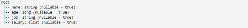
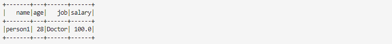
spark.sql(f"SELECT * FROM {table_name}.snapshots").show()

The above code shows schema evolution by renaming, changing column types, and adding a new column. As you can observe in the screenshots below, after and before schema evolution, the column age type has changed, the column job_title is now renamed to job, and the column salary has been added.

Apache Iceberg with PySpark — Schema before altering the table

The first time you run the code, in the snapshot table you notice that Iceberg executed all alterations without rewriting the data. This is indicated by having only one snapshot ID and no parent (parent_id = null), signifying that no data rewriting was performed.

How to use Apache Iceberg with PySpark — Snapshot table

Data accuracy and consistency are crucial in data lakes, particularly for business-critical purposes. Iceberg supports ACID transactions for write operations, ensuring that data remains in a consistent state, and enhancing the reliability of the stored information.

Transactional Writes

To demonstrate the ACID with Iceberg table let’s update, add, and delete records from the table.

spark.sql(f"UPDATE {table_name} SET salary = 100")
spark.sql(f"DELETE FROM {table_name} WHERE age = 42")
spark.sql(f"INSERT INTO {table_name} values ('person4', 50, 'Teacher', 2000)")
spark.sql(f"SELECT * FROM {table_name}.snapshots").show()

In the snapshots table, we can now observe that Iceberg has added three snapshot IDs, each created from the preceding one. If, for any reason, one of the actions fails, the transactions will fail, and the snapshot won’t be created.

Partitioning the table

As you may be aware, querying large amounts of data in data lakes can be resource-intensive. Iceberg supports data partitioning by one or more columns. This significantly improves query performance by reducing the volume of data read during queries.

spark.sql(f"ALTER TABLE {table_name} ADD PARTITION FIELD age")
spark.read.format("iceberg").load(f"{table_name}").where("age = 28").show()

The code creates a new partition using the age column. This partition will apply to the new rows that get inserted moving forward, and old data will not be impacted.

We can also add partitions when we create the Iceberg table using something like below.

spark.sql(f"""
        CREATE TABLE IF NOT EXISTS {table_name}
        (name STRING, age INT, job STRING, salary INT)
        USING iceberg
        PARTITIONED BY (age)
    """)

Time Travel

Analyzing historical trends or tracking changes over time is often essential in a data lake. Iceberg provides a time-travel API that allows users to query data as it appeared at a specific version or timestamp, facilitating historical data analysis.

Apache Iceberg gives you the flexibility to load any snapshot or data at a given point in time. This allows you to examine changes at a given time or roll back to a specific version.

spark.sql(f"SELECT * FROM {table_name}.snapshots").show(1, truncate=False)
# Read snapshot by id run
spark.read.option("snapshot-id", "306576903892976364").table(table_name).show()
# Read at a given time
spark.read.option("as-of-timestamp", "306576903892976364").table(table_name).show()

Query Isolation

Given the simultaneous use of data lakes by multiple users or applications, Iceberg allows for concurrent execution of multiple queries without mutual interference. This capability facilitates the scalability of data lake usage without compromising performance.

Conclusion

Apache Iceberg provides a robust solution for managing big data tables with features like atomic commits, schema evolution, and time travel. When combined with the power of PySpark, you can harness the capabilities of Iceberg while leveraging the flexibility and scalability of PySpark for your big data processing needs.

This article has provided a basic overview of using Apache Iceberg with PySpark, but there is much more to explore, including partitioning, indexing, and optimizing performance. For more in-depth information, refer to the official Apache Iceberg documentation.

You can find the complete source code for this article in my Github Repository.