[02] – Getting Started with Apache Iceberg

In this tutorial, you’ll learn how to install Apache Iceberg locally and get hands-on experience using Apache Spark as a compute engine.

First, we’ll set up the environment by creating a Python virtual environment and installing PySpark. Please note that some prior knowledge of PySpark is required to follow this tutorial.

Next, you’ll learn how to read and write PySpark DataFrames using Apache Iceberg.

Finally, you’ll explore Iceberg’s key features, including schema evolution, ACID transactions, time travel, and query isolation.

Prerequisites #

Before you start a PySpark session with Apache Iceberg, you will need to have the following installed:

• Java (v8 or v11)
• PySpark
• Apache Spark (the version depends on the Iceberg version)

Install required dependencies #

Before working with Apache Iceberg and PySpark, you’ll need to install the required dependencies. Use the following commands to create and activate a virtual environment (named iceberg, or any name you prefer), then install the pyspark package.

python -m venv iceberg
source iceberg/bin/activate
pip install pyspark==3.4.1

If you are using Windows, run the command .\iceberg\Scripts\activate to activate the virtual environment.

The versions used in this article are:

• Python: 3.11.6
• PySpark: 3.4.1

Import required packages #

Once you install the dependencies, import the necessary packages that you will use in the following sections.

from pyspark.sql import SparkSession
from pyspark import SparkConf
from pyspark.sql.types import StructType, StructField, StringType, IntegerType

Setup Iceberg Configuration #

To start working with Iceberg tables in PySpark, you first need to configure the PySpark session correctly. In this setup, you’ll use a catalog named demo that points to a local warehouse directory at ./warehouse, using the Hadoop catalog type.

The warehouse path acts as the storage location for all Iceberg table data and metadata. It’s essential for managing table state and ensuring consistent access across read/write operations.

Make sure the Iceberg-Spark Runtime JAR you use is compatible with your PySpark version. You can find the appropriate JAR files in the official Iceberg releases. For more advanced settings, refer to the Iceberg-Spark-Configuration documentation.

arehouse_path = "./warehouse"
iceberg_spark_jar  = 'org.apache.iceberg:iceberg-spark-runtime-3.4_2.12:1.3.0'
catalog_name = "demo"

# Setup iceberg config
conf = SparkConf().setAppName("YourAppName") \
    .set("spark.sql.extensions", "org.apache.iceberg.spark.extensions.IcebergSparkSessionExtensions") \
    .set(f"spark.sql.catalog.{catalog_name}", "org.apache.iceberg.spark.SparkCatalog") \
    .set('spark.jars.packages', iceberg_spark_jar) \
    .set(f"spark.sql.catalog.{catalog_name}.warehouse", warehouse_path) \
    .set(f"spark.sql.catalog.{catalog_name}.type", "hadoop")\
    .set("spark.sql.defaultCatalog", catalog_name) 

# Create spark session
spark = SparkSession.builder.config(conf=conf).getOrCreate()
spark.sparkContext.setLogLevel("ERROR")

With the Spark session now correctly configured, let’s move on to creating and reading an Iceberg table.

# Create a dataframe
schema = StructType([
    StructField('name', StringType(), True),
    StructField('age', IntegerType(), True),
    StructField('job_title', StringType(), True)
])
data = [("person1", 28, "Doctor"), ("person2", 35, "Singer"), ("person3", 42, "Teacher")]
df = spark.createDataFrame(data, schema=schema)

# Create database
spark.sql(f"CREATE DATABASE IF NOT EXISTS db")

# Write and read Iceberg table
table_name = "db.persons"
df.write\
  .format("iceberg")\
  .mode("overwrite")\
  .saveAsTable(f"{table_name}")

iceberg_df = spark.read\
  .format("iceberg")\
  .load(f"{table_name}")

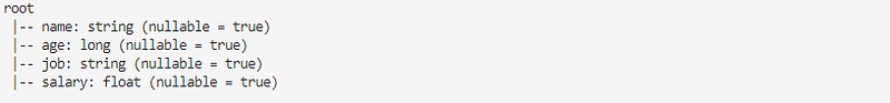
iceberg_df.printSchema()
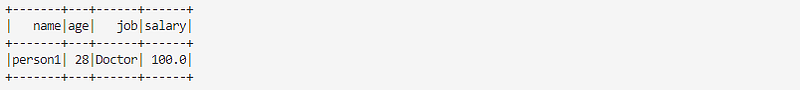
iceberg_df.show()

In the code above, we created a PySpark DataFrame, wrote it to an Iceberg table db.persons, and then read the data back for display.

Now, let’s explore the key features of Iceberg that help solve the challenges outlined in the introduction.

Schema Evolution #

Data lakes support various data formats, but that flexibility often makes schema management a challenge. Iceberg addresses this by allowing you to add, remove, or modify columns without rewriting the entire dataset — making schema evolution seamless and efficient.

Let’s update the existing table db.personsto demonstrate how schema evolution works in practice.

Data lakes support a wide range of data formats, but that flexibility can make schema management difficult. Iceberg solves this by allowing columns to be added, removed, or modified without rewriting the entire dataset. This makes it much easier to evolve schemas over time.

spark.sql(f"ALTER TABLE {table_name} RENAME COLUMN job_title TO job")
spark.sql(f"ALTER TABLE {table_name} ALTER COLUMN age TYPE bigint")
spark.sql(f"ALTER TABLE {table_name} ADD COLUMN salary FLOAT AFTER job")
iceberg_df = spark.read.format("iceberg").load(f"{table_name}")
iceberg_df.printSchema()
iceberg_df.show()

spark.sql(f"SELECT * FROM {table_name}.snapshots").show()

The code above demonstrates schema evolution with three operations:

• Renaming a column
• Changing a column’s data type
• Adding a new column

As shown in the screenshots below, job_title has been renamed to job, the age column’s type has been updated, and a new column, salary, has been added.

The first time you run the code, in the snapshot table you notice that Iceberg executed all alterations without rewriting the data. This is indicated by having only one snapshot ID and no parent (parent_id = null), signifying that no data rewriting was performed.

ACID transactions #

Data accuracy and consistency are crucial in data lakes, particularly for business-critical purposes. Iceberg supports ACID transactions for write operations, ensuring that data remains in a consistent state, and enhancing the reliability of the stored information.

To demonstrate the ACID with Iceberg table let’s update, add, and delete records from the table.

spark.sql(f"UPDATE {table_name} SET salary = 100")
spark.sql(f"DELETE FROM {table_name} WHERE age = 42")
spark.sql(f"INSERT INTO {table_name} values ('person4', 50, 'Teacher', 2000)")
spark.sql(f"SELECT * FROM {table_name}.snapshots").show()

In the snapshots table, we can now observe that Iceberg has added three snapshot IDs, each created from the preceding one. If, for any reason, one of the actions fails, the transactions will fail, and the snapshot won’t be created.

Partition Evolution #

As you may be aware, querying large amounts of data in data lakes can be resource-intensive. Iceberg supports data partitioning by one or more columns. This significantly improves query performance by reducing the volume of data read during queries.

spark.sql(f"ALTER TABLE {table_name} ADD PARTITION FIELD age")
spark.read.format("iceberg").load(f"{table_name}").where("age = 28").show()

The code creates a new partition based on the age column. This partitioning applies only to new rows inserted after the change; existing data remains unaffected.

You can also define partitions at table creation time using the PARTITIONED BY clause, as shown below.

spark.sql(f"""
        CREATE TABLE IF NOT EXISTS {table_name}
        (name STRING, age INT, job STRING, salary INT)
        USING iceberg
        PARTITIONED BY (age)
    """)

Time Travel #

Analyzing historical trends or tracking changes over time is a common need in data lakes. Iceberg addresses this with its time travel feature, allowing users to query data as it existed at a specific snapshot or timestamp.

This capability lets you:

• Load any historical version of a table
• Examine how data changed over time
• Roll back to a previous state if needed

Iceberg’s time-travel API makes it easy to perform audits, recover from errors, or support reproducible analysis based on past data states.

# List snapshots
spark.sql(f"SELECT * FROM {table_name}.snapshots").show(1, truncate=False)

# Read snapshot by id run
spark.read.option("snapshot-id", "306576903892976364").table(table_name).show()

# Read at a given time
spark.read.option("as-of-timestamp", "306576903892976364").table(table_name).show()

The code above Iceberg’s time travel feature. The first line queries the table’s snapshot metadata to list available snapshots. The second line reads the table as it existed at a specific snapshot ID. The third line reads the table as it was at a specific point in time, using a timestamp.